Wind Forecasting
Evaluating neural and classical models for multi-horizon wind prediction
Three recurrent architectures trained to correct numerical weather forecasts at +24, +48 and +72 hours, measured against a gradient-boosted baseline that beat all of them.
- +24 h MAE, trees against BiLSTM
- 2.76 vs 2.86
- km/h, 748 shared targets; the baseline wins
- +48 h MAE, trees against BiLSTM
- 3.08 vs 3.22
- km/h, same targets
- +72 h MAE, trees against BiLSTM
- 3.11 vs 3.30
- km/h, same targets
- BiLSTM gain over the raw forecast
- 17.3 / 14.2 / 9.8%
- MAE at +24 / +48 / +72 h; the network does correct the bulletin
Figures with a dotted underline carry their source. Hover one to see whether it was verified in code or reported in project documentation.
Context
The situation
A numerical weather model forecasts a grid cell, not a site. The gap between the two is systematic and learnable, which is what makes local correction a reasonable supervised problem rather than a repeat of meteorology.
The problem
Forecasting problems make it very easy to fool yourself. Random splits leak the future into training; a persistence baseline is trivially beatable and tells you nothing; and the test set gets looked at long before the model is finished. Each of those produces a number that looks good and means nothing.
What I built
Fix the protocol before the model. Split by time, select on 2025, calibrate intervals on late 2025, and score once on January 2026. Compare against two baselines that are hard rather than convenient: the raw numerical forecast, and gradient-boosted trees on the same inputs. Train three recurrent architectures with two seeds each, commit the selection before computing test scores, and keep the ablation that fails.
Numerical weather prediction gives you a wind forecast for a region. What a specific site needs is a local correction to it. This trains recurrent networks to learn that correction at three lead times, using six years of hourly Météo-France station observations and archived forecasts from four numerical models. Three architectures were trained with two seeds each and selected on 2025 validation before the 2026 test month was scored. The selected BiLSTM cuts the raw forecast error by 17.3, 14.2 and 9.8 percent at +24, +48 and +72 hours, and loses to a gradient-boosted baseline at all three.
Architecture
How it fits together
- Station observationsinput
hourly, 2020 to 2026
- Archived forecastsinput
ECMWF, ICON Global, ICON Europe, GFS
- Causal sequencesdeterministic
72 h history, masks, purged boundaries
- Temporal splitguard
select 2025, calibrate late 2025, test 2026
- Recurrent candidateslanguage model
BiGRU, BiLSTM, attention, ablation
- Boosted baselinelanguage model
the model that has to be beaten
- Scored onceoutput
748 shared targets per lead time
Key decisions
The choices that shaped it
- 01
Choose a baseline that can win
The earlier version of this project compared a GRU against persistence and beat it by 1.1 percent MAE. Persistence is not a serious opponent at a 24 hour horizon, so that number said almost nothing. The current work measures against the raw numerical forecast and against gradient-boosted trees on the same inputs, and the trees win. That is a far more informative result than the one it replaced.
- 02
Commit the selection before scoring the test
The candidate architecture and its epochs were chosen on 2025 validation and committed to the repository before the 2026 scores were computed. Without that ordering, choosing the best of three architectures after seeing test numbers is just a slower way of fitting the test set.
reports/wind_neural/selection.json
- 03
Say that the test month had already been seen
The January 2026 window had been looked at during earlier work, so the comparison is retrospective on a reused and wintry test set. The repository states this in the README, in the metrics artefact and on the chart itself. A reused test set is a weaker claim and pretending otherwise would be the easiest lie available here.
reports/wind_neural/metrics.json
- 04
Keep the ablation that disproves the idea
A control neutralises the input sequence while keeping the context’s history variables. If the recurrent sequence were carrying the signal, that control should fall behind. It does not clearly do so, which means the extra sequence is not demonstrably contributing. Attention does not improve validation either. Both negative results are kept in the repository and on the chart.
- 05
Give the forecast an availability margin
Archived numerical forecasts are indexed by initialisation time rather than actual publication time, so using them naively assumes a bulletin was available the instant it was computed. The pipeline conservatively uses 48, 72 and 96 hour archive offsets for the 24, 48 and 72 hour predictions, allowing a full day for availability, and applies the same restriction to the reference it is compared against.
- 06
Report interval coverage, not just the nominal level
Prediction intervals were calibrated on late 2025 at a nominal 80 percent. Observed coverage on the test month is 79.4, 76.3 and 76.7 percent at the three horizons. The chart prints the observed figures next to the nominal one and states that the nominal level is not a guarantee.
Evidence
What it actually looked like
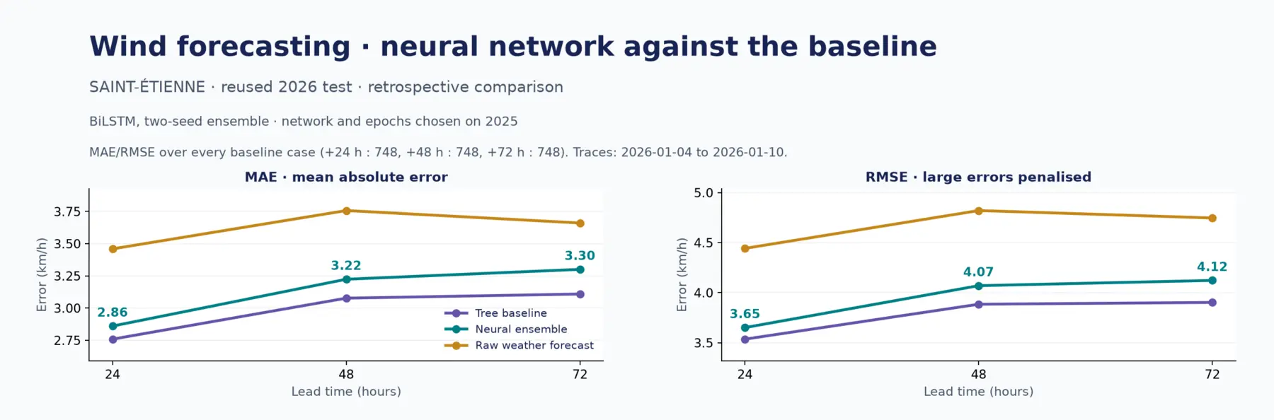
The measured result. The network corrects the raw bulletin at every horizon and still sits above the tree baseline at every horizon.
Figure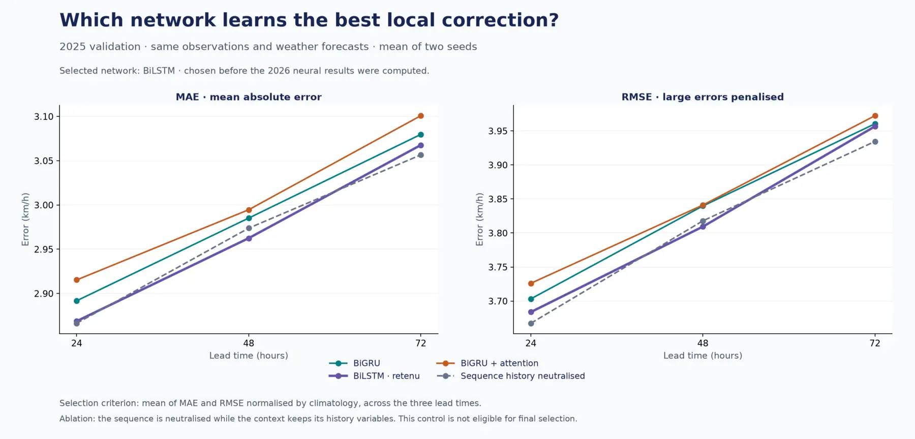
Candidate selection on 2025 validation, committed before the test month was scored. Attention does not help, and the sequence ablation does not clearly fall behind.
FigureMeasured
Every figure, with its source
- +24 h MAE, trees against BiLSTM
- 2.76 vs 2.86
- km/h, 748 shared targets; the baseline wins
- +48 h MAE, trees against BiLSTM
- 3.08 vs 3.22
- km/h, same targets
- +72 h MAE, trees against BiLSTM
- 3.11 vs 3.30
- km/h, same targets
- BiLSTM gain over the raw forecast
- 17.3 / 14.2 / 9.8%
- MAE at +24 / +48 / +72 h; the network does correct the bulletin
- Architectures and seeds
- 3 × 2
- BiGRU, BiLSTM, BiGRU with attention, plus a sequence-neutralised control
- Tests, and replay tolerance
- 32 tests
- historical issue-time replay reproduces saved predictions to 1e-4 km/h
Figures with a dotted underline carry their source. Hover one to see whether it was verified in code or reported in project documentation.
My contribution
Sole author. Data pipeline, models, protocol, evaluation and reporting.
What I owned
- Causal sequence construction: hourly reindexing, missing-target masks, normalisations fitted on training data only, temporal boundaries purged out to +72 h
- Three architectures, BiGRU, BiLSTM and BiGRU with attention, plus a control that neutralises the sequence while keeping history variables
- A pre-registered protocol: candidate and epoch selection committed before the test month was scored
- Gradient-boosted and linear baselines over ECMWF, ICON Global, ICON Europe and GFS forecast inputs
- Calibrated prediction intervals, with observed coverage reported against the nominal level
- Historical issue-time replay that reproduces saved predictions to 1e-4 km/h, and 32 unit tests covering causality, models and training
Stack and limits
Built with
- Python
- PyTorch
- pandas
- scikit-learn
- LightGBM
- matplotlib
Techniques
- Recurrent sequence models
- Multi-horizon direct forecasting
- Temporal validation and embargo
- Pre-registered model selection
- Interval calibration and coverage
- Ablation controls
What it is not
- The tree baseline wins at all three horizons. The recurrent model is the second-best method here and the page says so.
- The test window is one winter month that had already been looked at during earlier work, which makes the comparison retrospective and weaker than a clean holdout.
- One station, Saint-Étienne. Nothing here measures whether the correction transfers to another site or another season.
- Outputs are wind speed only, not gusts and not direction.
- Prediction intervals undershoot their nominal 80 percent level at the longer horizons.
- Replay works on archived data. There is no live forecasting service.
What carried forward
The first version of this beat a persistence baseline by one percent and I was pleased with it. Replacing persistence with the model a practitioner would actually use turned a small win into a clear loss, and that is the more useful artefact. Most of the value in a forecasting project sits in the protocol, not the architecture.
Next
April to October 2026
Agent Fabric
A 1.39 million node graph of pull requests, people and repositories, built to test one question: does relational structure beat hand-built features? The experiment is designed so that it can say no.
Read case study→June 2026
Geometry-aware world models for EEG
EEG channel covariance lives on a curved manifold. I built three prediction heads to test whether the geometry matters. It did not, and proving that cleanly was the contribution.
Read case study→