June 2026Hack the World(s) 2026 · Paris

Geometry-aware world models for EEG

Self-supervised representation learning, and an honest null

Three prediction heads in three geometries on a shared EEG encoder, plus the multi-seed cluster ablations behind a study whose headline result was a clean null.

One of four — owned the world-model trackView source ↗View architecture

Frozen linear probe, balanced accuracy: 0.819; team result · 3 seeds · patient-disjoint split
AUROC: ~0.89; 3-seed mean
Random-encoder floor: ~0.79; disclosed against our own headline
Ablation spread across the 2×2: ≤ 0.013; a clean null, 3 seeds per cell

Figures with a dotted underline carry their source. Hover one to see whether it was verified in code or reported in project documentation.

Context

The situation

EEG channel covariance is a symmetric positive-definite matrix, so it lives on a curved manifold rather than in flat Euclidean space. Self-supervised methods routinely apply their anti-collapse regulariser in the ambient space anyway.

The problem

Where should the anti-collapse regulariser act — in plain Euclidean space, or in the tangent space of the SPD manifold where the data actually lives? And does acting in the correct geometry buy anything measurable?

What I built

A controlled study rather than a leaderboard attempt. Pretrain, freeze, then linear-probe on held-out patients, which is the honest test of what pretraining contributed. Cross two regularisers with two spaces, run three seeds per cell, and disclose the floor a random untrained encoder reaches in the same pipeline.

Self-supervised encoders are usually judged after fine-tuning, which hides how much the pretraining actually contributed. Our team pretrained a two-view encoder on unlabelled EEG, froze it, and linear-probed abnormality on a patient-disjoint split, running a controlled 2×2 of regulariser against geometry across three seeds. I owned the world-model track: three parallel prediction heads on a shared encoder — ambient Euclidean, Log-Euclidean tangent, and full log-SPD Riemannian — plus the six-class event transfer pipeline. Every cell of the ablation landed near the same accuracy. Geometry helped neither accuracy nor calibration, and my own three-geometry model lost to the simple baseline.

Architecture

How it fits together

Raw EEG windowsinput
unlabelled, two augmented views
Shared encoderdeterministic
1-D convolutional
Ambient headlanguage model
Euclidean · isotropic-Gaussian target
Tangent headlanguage model
Log-Euclidean · distribution-free
Riemannian headlanguage model
full log-SPD · variance-covariance
Freezeguard
no fine-tuning
Linear probeoutput
held-out patients

One shared encoder, three prediction heads, three geometries. Each head pairs with the anti-collapse objective whose distributional assumption actually holds in that space.

Key decisions

The choices that shaped it

Each of these was a fork in the road where the obvious option would have produced something that looked the same and behaved worse.

01
Pair each geometry with an objective whose assumptions hold there
The ambient head uses an isotropic-Gaussian anti-collapse target, which is reasonable in flat space. Tangent vectors of an SPD manifold are not Gaussian, so the tangent head uses a distribution-free regulariser instead. Applying the Gaussian objective everywhere would have confounded geometry with mis-specification.
02
Log-Euclidean, for numerical stability
The full-matrix Riemannian head initially diverged. Moving to the Log-Euclidean metric — a valid Riemannian metric on SPD matrices that linearises the space through the matrix logarithm — plus gradient clipping made it trainable.
03
Freeze, then probe
Fine-tuning conflates what pretraining learned with what the downstream head learned. Freezing the encoder and fitting a linear probe on patient-disjoint recordings measures the representation itself, which is the only question the study was asking.
04
Disclose the random-encoder floor
A randomly initialised, untrained encoder reaches roughly 0.79 balanced accuracy in the same pipeline, because EEG abnormality is largely power-driven and random convolutional filters preserve band power. Reporting that reframes the headline from “strong” to “a quantified increment over a floor” — and implies that several published frozen foundation-model numbers barely clear a random baseline.
05
Report the null, and report losing
The 2×2 came out flat: every cell landed near the same accuracy, with gaps below a plausible bootstrap interval. My own three-geometry world model then lost to the simple baseline on the event-transfer task, and the effective-rank diagnostic explained why. Both results are in the write-up.

Evidence

What it actually looked like

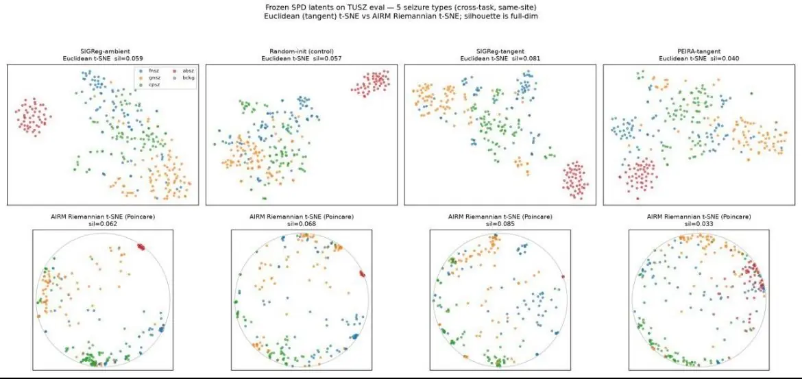
Frozen linear-probe balanced accuracy on held-out patients. Our in-domain result reaches 0.819 and our general-pretrained result 0.814, above every frozen foundation-model row quoted from EEG-FM-Bench — and above our own random-initialised encoder at 0.790, which is drawn on the same axis. — The frozen head-to-head. Our rows are measured locally; the foundation-model rows are quoted. The random-encoder floor at 0.790 is on the same chart, because leaving it off would make the result look like something it is not.
Figure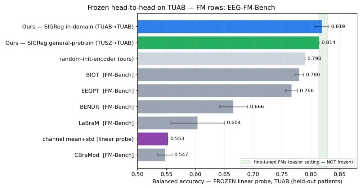

Latent structure under four training configurations, projected two ways: a t-SNE of the Euclidean embedding on top, and a Riemannian t-SNE on the Poincaré disc below, with points coloured by seizure event type. — Where the geometry did show up. The probe numbers barely move between configurations; the latent structure visibly does.
Figure

Measured

Every figure, with its source

Frozen linear probe, balanced accuracy: 0.819; team result · 3 seeds · patient-disjoint split
AUROC: ~0.89; 3-seed mean
Random-encoder floor: ~0.79; disclosed against our own headline
Ablation spread across the 2×2: ≤ 0.013; a clean null, 3 seeds per cell
Evaluation split: 2717 / 276; train / eval recordings, patient-disjoint

Figures with a dotted underline carry their source. Hover one to see whether it was verified in code or reported in project documentation.

Recognition

Result

FinalistHack the World(s) 2026Paris

World Models & JEPA Hackathon · under the patronage of Yann LeCun

25 teams · 100 selected participants · 650+ applicants

A 24-hour hackathon on world models, held under the patronage of Yann LeCun, who gave the opening keynote. One hundred students were selected from more than 650 applications and competed in 25 teams of four.

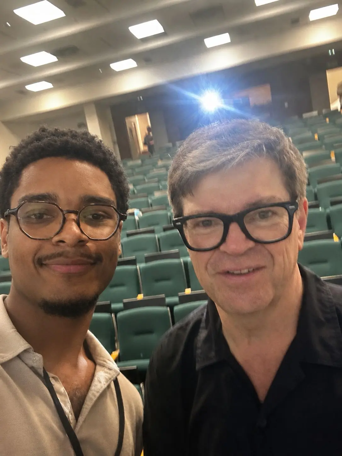
The opening keynote at Hack the World(s) 2026, in a full lecture theatre, with Yann Le Cun’s name on the screen. — The opening keynote. The event ran under Yann LeCun’s patronage.
Event

The result is context. What the system does, and how it was measured, is everything above this.

My contribution

One of four. Owned the world-model track, the event-transfer pipeline and the results figures.

What I owned

A three-geometry world model: parallel prediction heads in ambient Euclidean, Log-Euclidean tangent (upper-triangular log-SPD) and full-matrix Riemannian space, each paired with the anti-collapse objective appropriate to its distribution
Stabilising the Riemannian head with a Log-Euclidean metric and gradient clipping
The six-class event pipeline end to end: dataset, evaluation, training config, cluster job and loss logging
An asymmetric variant with an EMA target encoder and latent predictor, as a contrast to the team’s symmetric objective
The single-view versus two-view ablation
The results-figure pipeline turning cluster logs into the deck’s figures, including the collapse diagnostic

What I did not

The repository lead and the majority of its commits
The core 2×2 regulariser study and the headline frozen-probe number
The graph-JEPA and spectral encoder tracks

Team

Stack and limits

Built with

Python
PyTorch
NumPy
SLURM
OmegaConf
matplotlib

Techniques

Joint-embedding predictive architectures
SPD manifold geometry · matrix logarithm · Log-Euclidean metric
Anti-collapse regularisation
Frozen linear probing
Effective-rank collapse diagnostics
Multi-seed cluster ablations

What it is not

Not a foundation model, not state of the art, and framed throughout as a controlled transfer study.
The headline balanced accuracy is the team’s core result. My own world-model track underperformed that baseline on the transfer task.
The study vendors an existing open-source EEG dataloader and two of its loss implementations, which are reused intact.
One arm of the comparison ran at a single seed rather than three.

What carried forward

The most useful output was not a number but a habit: publish the floor that shrinks your own result. A frozen-probe benchmark where random convolutional filters reach 0.79 is a benchmark measuring band power, and that is worth saying out loud even when it makes your own headline smaller.

July – August 2026

Omnivision

Assistive tools describe scenes but carry no memory, and cannot tell recognising something from being confident about it. I built the part that refuses.

Read case study→

July 2026

Obligation Ledger

The model proposes a termination date. The service throws it away and recomputes it from verified quotes. Nothing is approvable until every value has been found on its page.