Agent Fabric
Temporal graph learning for software and operational systems
Models software delivery as a temporal heterogeneous graph and asks whether graph learning actually predicts delivery outcomes better than simpler models. The honest answer is: barely, and at two hundred times the cost.
- Graph size
- 1.39M nodes
- 816k pull requests, 547k users, 24k repositories; 12.4M directed edges
- HeteroSAGE vs MLP, intrinsic features
- 0.678→0.721
- +0.043 AUC, paired 95% CI [0.037, 0.049]
- Best graph model over LightGBM, both with history
- +0.0075
- 0.730 against 0.722, CI [0.004, 0.011]
- Training cost of that gain
- ~200×
- 87s for HeteroSAGE against 0.4s for LightGBM, on four CPU cores
Figures with a dotted underline carry their source. Hover one to see whether it was verified in code or reported in project documentation.
Context
The situation
Coding agents see the code, the tickets and the docs, but not the causal history that produced them. The question underneath is whether that history is learnable from structure, or whether a few well-chosen features capture it just as well.
The problem
Relational learning is easy to justify in a slide and hard to justify in a benchmark. A graph model will almost always beat a weak baseline. The experiment is only worth running if the baseline is the one a practitioner would actually reach for, and if the setup cannot leak the answer.
What I built
Build the graph properly, then try hard to beat it with something cheaper. Nodes are pull requests, users and repositories; every edge carries the time of its interaction and has a reverse twin, giving 32 edge types. Users and repositories are deliberately featureless, so their state has to be reconstructed from the time-filtered neighbourhood. Then run MLP, HeteroSAGE and HGT against logistic regression and LightGBM, with and without point-in-time history aggregates, three seeds each, paired bootstrap confidence intervals on the same test seeds.
When a pull request is opened, will it be merged within 48 hours? Whether it lands plausibly depends on the author’s track record, the repository’s habits and the reviewers’ activity, none of which live inside the pull request. That makes it a natural test of relational learning, so the project builds a temporal heterogeneous graph over three weeks of public GitHub events and compares graph neural networks against gradient boosting on point-in-time aggregates. The graph does recover the history signal on its own, worth +0.043 AUC over an identical MLP. On top of hand-built aggregates it adds +0.0075, for roughly two hundred times the training cost.
Architecture
How it fits together
- GH Archiveinput
hourly events, streamed
- Typed eventsdeterministic
Parquet, never stored raw
- Temporal graphdeterministic
1.39M nodes, 12.4M edges, 32 edge types
- Temporal samplingguard
no edge newer than the seed
- MLP / HeteroSAGE / HGTlanguage model
same loop, same splits
- LogReg / LightGBMlanguage model
the baseline that has to be beaten
- Paired comparisonoutput
3 seeds, bootstrap CIs on shared test seeds
Key decisions
The choices that shaped it
- 01
Make the baseline strong on purpose
The interesting comparison is not against a weak model. LightGBM gets the same point-in-time history aggregates a practitioner would build by hand, computed strictly before each pull request opened. With those features it reaches 0.722 AUC, which is within 0.008 of the best graph model. Running the experiment against a weaker baseline would have produced a much more flattering and much less useful result.
training/tabular_baselines.py
- 02
Three leakage controls, each with a test
Temporal neighbour sampling never returns an edge newer than the seed pull request’s open time, so a pull request cannot see its own merge or its own reviews. Node features are point-in-time. Train, validation and test are split by time with an embargo, so every label in a split resolves before the next split begins. Each of the three has a test, because leakage in a temporal graph is silent and flatters you.
- 03
Featureless users and repositories, deliberately
User and repository nodes carry no features at all. Their state changes over time, so attaching a static feature vector would either be stale or leak. Instead their state is reconstructed from the time-filtered neighbourhood, which is the thing the graph is supposed to be good at. It also makes the comparison honest: the graph has to earn the history signal rather than being handed it.
- 04
The graph recovers the signal, then stops paying for itself
On intrinsic features alone, HeteroSAGE beats an identical-loop MLP by +0.043 AUC with a paired 95% interval of [0.037, 0.049]. That is almost exactly the lift hand-built history aggregates give LightGBM, +0.042. So the structure genuinely contains the history. On top of those aggregates it adds a further +0.0075, significant but small, for roughly two hundred times LightGBM’s training time on CPU. The repository says plainly that a gradient-boosted tree on point-in-time aggregates is the sensible default for this task today.
experiments/results/gh_pr_merge__main.md
- 05
HGT is not better than the cheaper model
HGT trains about 1.9 times slower than HeteroSAGE and scores slightly below it, −0.0054 with a paired interval of [−0.0082, −0.0024]. The more expressive architecture is not the better one here, and reporting that was more useful than quietly keeping only the best row.
- 06
Self-supervised pretraining helps exactly where you would expect
A temporal JEPA objective pretrains the encoder without labels. Under a linear probe it beats a random frozen encoder, 0.696 against 0.651, and on real data that frozen representation matches a supervised HGT trained on 10% of the labels. With all labels it is neutral on real data and actively hurts on synthetic data. Useful when labels are scarce, pointless when they are not.
- 07
Two upstream defects, found by measurement rather than by reading
PyTorch Geometric’s HGTConv builds its relation type vector in the iteration order of the edge dictionary, then feeds it to a linear layer that assumes the vector is sorted. When the two orders disagree, which is the normal case once forward and reverse relations are inserted pairwise, relation-specific key and value weights are applied to the wrong node segments silently. It only surfaced because a timing cache eventually selected a different kernel and crashed on negative split sizes. Both HGT wrappers now pass edges in metadata order, a regression test documents the upstream behaviour, and a report is drafted. The cuGraph-PyG temporal leakage below is the second.
test_pyg_hgtconv_is_order_sensitive_and_our_wrapper_is_not
- 08
The GPU sampler runs, leaks, and is slower
cuGraph-PyG was made to work on a laptop GTX 1650 Max-Q after seven workarounds. Then measurement killed it: two-hop temporal sampling is not leakage-safe, with about 0.7 to 0.9% of sampled edges newer than their seed and roughly 2% of batches carrying out-of-range indices. It was excluded from training and a draft upstream bug report written instead. Moving the model to the GPU did help, speeding HGT up three to five times, but the GPU sampler itself was 5.8 times slower than pyg-lib on four CPU cores.
experiments/results/cugraph_temporal_check.json
Evidence
What it actually looked like
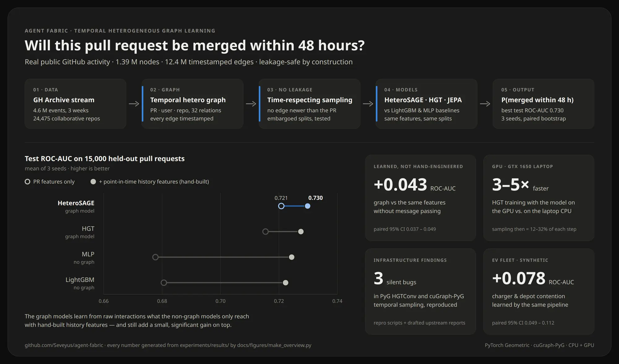
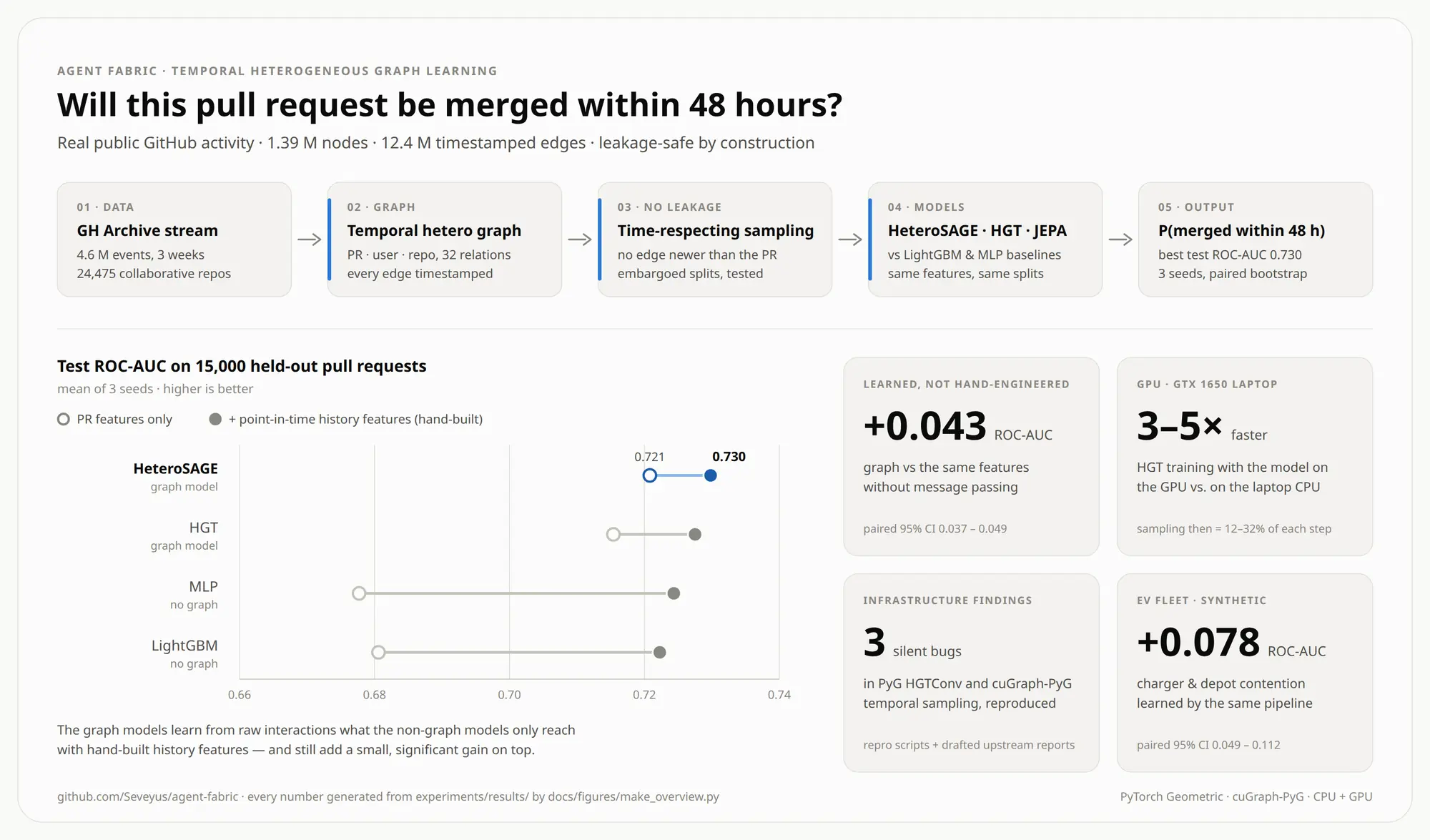
Generated from experiments/results by a script in the repository, so the figure cannot drift from the numbers it reports. The dumbbells show each model twice: intrinsic features, then with hand-built history. The graph models start where the others finish.
FigureMeasured
Every figure, with its source
- Graph size
- 1.39M nodes
- 816k pull requests, 547k users, 24k repositories; 12.4M directed edges
- HeteroSAGE vs MLP, intrinsic features
- 0.678→0.721
- +0.043 AUC, paired 95% CI [0.037, 0.049]
- Best graph model over LightGBM, both with history
- +0.0075
- 0.730 against 0.722, CI [0.004, 0.011]
- Training cost of that gain
- ~200×
- 87s for HeteroSAGE against 0.4s for LightGBM, on four CPU cores
- JEPA linear probe vs random frozen encoder
- 0.651→0.696
- real graph; the gain disappears once all labels are available
- cuGraph two-hop temporal sampling
- not leakage-safe
- ~0.7 to 0.9% of sampled edges newer than their seed; excluded from training
Figures with a dotted underline carry their source. Hover one to see whether it was verified in code or reported in project documentation.
My contribution
Sole author of the graph-learning pipeline, models, experiments and benchmarks.
What I owned
- GH Archive ingestion into typed Parquet events, streamed rather than stored raw
- The temporal heterogeneous graph: 32 edge types, point-in-time node features, time-based splits with an embargo
- Three leakage controls, each with its own test: temporal neighbour sampling, point-in-time features, embargoed splits
- MLP, HeteroSAGE and HGT, plus logistic regression and LightGBM baselines on the same splits
- A temporal JEPA objective, evaluated by linear probe and by fine-tuning at 10% and 100% of labels
- Two interchangeable sampling backends behind one interface, PyG on CPU and cuGraph-PyG on GPU
- Multi-seed suites with paired bootstrap confidence intervals, and a synthetic EV-fleet transfer check
Stack and limits
Built with
- Python
- PyTorch
- PyTorch Geometric
- pyg-lib
- cuGraph-PyG
- LightGBM
- Parquet
- FastAPI
Techniques
- Temporal heterogeneous graphs
- HeteroSAGE and HGT
- Joint-embedding predictive pretraining
- Leakage-safe temporal sampling
- Paired bootstrap confidence intervals
- GPU sampling backends
What it is not
- The graph gain beyond engineered aggregates is +0.005 to +0.0075 AUC at a large compute cost. On this task, gradient boosting on point-in-time aggregates is the sensible default.
- One window: three weeks of September 2025, one temporal test window, 24,475 pre-selected repositories, subsampled seeds. Stability over time is not measured.
- GitHub trimmed its public event payloads in October 2025, so later data cannot support this task at all.
- GPU evidence comes from one laptop. The cuGraph backend runs but is not leakage-safe at two hops and was slower than CPU sampling there.
- The EV-fleet transfer check runs on a synthetic depot simulator, not real fleet data. It shows the pipeline carries over, not that it works on a real fleet.
- The platform’s pre-flight endpoint scores consequences with hand-set heuristics. The trained graph models are not deployed behind it.
- No temporal encoding beyond sampling, no calibration, no per-prediction explanations.
What carried forward
The result I expected was that the graph would win. It does, and the margin is small enough that the honest recommendation is to use the cheaper model. Designing the experiment so it could say that, with a baseline strong enough to actually threaten the hypothesis and leakage controls tight enough to trust the gap, was most of the work.
Next
June 2026
Geometry-aware world models for EEG
EEG channel covariance lives on a curved manifold. I built three prediction heads to test whether the geometry matters. It did not, and proving that cleanly was the contribution.
Read case study→March to September 2026
Wind Forecasting
The BiLSTM improves on the raw weather forecast by up to 17%. It still loses to boosted trees at every horizon. The project is kept because that is the result.
Read case study→